Possible STARDIS Outputs
Import Necessary Code
[5]:
import numpy as np
import matplotlib.pyplot as plt

from stardis.base import run_stardis

from astropy import units as u, constants as const
Selecting Result Options
STARDIS simulations contain a variety of information, and depending on your needs you can have different parts of a simulation returned.
There are three parts of the simulation you can choose to return:
Stellar_Model
Stellar_Plasma
Stellar_Radiation_Field
Regardless of which are set to return, the simulation will always produce the stellar spectrum (such as the one displayed in the quickstart notebook).
To access these different parts of the model, you need to declare what you want to be returned in your configuration YAML file. This notebook uses a YAML file named stardis_outputs_config.yml which has the following lines:
        ...
no_of_thetas: 20
result_options: # <-----
    return_model: True # <----- defaults to False
    return_plasma: True # <----- defaults to False
    return_radiation_field: True # <----- defaults to True
Creating Example Simulation
[6]:
tracing_lambdas = np.mgrid[6540:6590:.01]* u.Angstrom

sim = run_stardis('stardis_outputs_config.yml', tracing_lambdas)
WARNING: UnitsWarning: 'erg/cm2/s' contains multiple slashes, which is discouraged by the FITS standard [astropy.units.format.generic]
Stellar Model
The stellar model is based on the information derived from the MARCS file for your star, and you can access it to verify STARDIS correctly processed the file. In the below example we are using the stellar model to look at simulated depths in our star in centimeters.
[7]:
sim.stellar_model.geometry.r
[7]:
Stellar Plasma
The stellar plasma is generated from the stellar model, and in it we can find information about the makeup and qualities of the plasma in our simulated star. Here is an example of us looking at the density of ions at different depths within our star.
[8]:
sim.stellar_plasma.ion_number_density
[8]:
| 0 | 1 | 2 | 3 | 4 | 5 | 6 | 7 | 8 | 9 | ... | 46 | 47 | 48 | 49 | 50 | 51 | 52 | 53 | 54 | 55 | ||
|---|---|---|---|---|---|---|---|---|---|---|---|---|---|---|---|---|---|---|---|---|---|---|
| atomic_number | ion_number | |||||||||||||||||||||
| 1 | 0 | 1.357488e+17 | 1.321919e+17 | 1.295592e+17 | 1.277547e+17 | 1.267249e+17 | 1.264809e+17 | 1.267312e+17 | 1.272488e+17 | 1.280748e+17 | 1.292835e+17 | ... | 3.966417e+15 | 3.116191e+15 | 2.447204e+15 | 1.920907e+15 | 1.507041e+15 | 1.181611e+15 | 9.258287e+14 | 7.247400e+14 | 5.667448e+14 | 4.413455e+14 |
| 1 | 6.385172e+15 | 5.006329e+15 | 3.898646e+15 | 2.999333e+15 | 2.260427e+15 | 1.644337e+15 | 1.367509e+15 | 1.110215e+15 | 8.708180e+14 | 6.501580e+14 | ... | 3.478357e+09 | 2.392115e+09 | 1.629784e+09 | 1.100527e+09 | 7.368918e+08 | 4.895196e+08 | 3.230976e+08 | 2.125878e+08 | 1.401980e+08 | 9.814634e+07 | |
| 2 | 0 | 1.209755e+16 | 1.167746e+16 | 1.135911e+16 | 1.112897e+16 | 1.097843e+16 | 1.090522e+16 | 1.090297e+16 | 1.092512e+16 | 1.097505e+16 | 1.105915e+16 | ... | 3.375972e+14 | 2.652311e+14 | 2.082910e+14 | 1.634958e+14 | 1.282700e+14 | 1.005715e+14 | 7.880083e+13 | 6.168539e+13 | 4.823782e+13 | 3.756461e+13 |
| 1 | 6.058951e+09 | 3.353671e+09 | 1.817801e+09 | 9.521732e+08 | 4.719585e+08 | 2.133037e+08 | 1.343820e+08 | 7.961535e+07 | 4.322331e+07 | 2.071727e+07 | ... | 4.557768e-04 | 2.346949e-04 | 1.187835e-04 | 5.913624e-05 | 2.898587e-05 | 1.400182e-05 | 6.683730e-06 | 3.172236e-06 | 1.512106e-06 | 8.051582e-07 | |
| 2 | 5.581645e-13 | 7.050644e-14 | 8.127889e-15 | 8.158929e-16 | 6.613797e-17 | 3.784828e-18 | 7.112620e-19 | 1.065274e-19 | 1.157150e-20 | 0.000000e+00 | ... | 0.000000e+00 | 0.000000e+00 | 0.000000e+00 | 0.000000e+00 | 0.000000e+00 | 0.000000e+00 | 0.000000e+00 | 0.000000e+00 | 0.000000e+00 | 0.000000e+00 | |
| ... | ... | ... | ... | ... | ... | ... | ... | ... | ... | ... | ... | ... | ... | ... | ... | ... | ... | ... | ... | ... | ... | ... |
| 30 | 26 | 0.000000e+00 | 0.000000e+00 | 0.000000e+00 | 0.000000e+00 | 0.000000e+00 | 0.000000e+00 | 0.000000e+00 | 0.000000e+00 | 0.000000e+00 | 0.000000e+00 | ... | 0.000000e+00 | 0.000000e+00 | 0.000000e+00 | 0.000000e+00 | 0.000000e+00 | 0.000000e+00 | 0.000000e+00 | 0.000000e+00 | 0.000000e+00 | 0.000000e+00 |
| 27 | 0.000000e+00 | 0.000000e+00 | 0.000000e+00 | 0.000000e+00 | 0.000000e+00 | 0.000000e+00 | 0.000000e+00 | 0.000000e+00 | 0.000000e+00 | 0.000000e+00 | ... | 0.000000e+00 | 0.000000e+00 | 0.000000e+00 | 0.000000e+00 | 0.000000e+00 | 0.000000e+00 | 0.000000e+00 | 0.000000e+00 | 0.000000e+00 | 0.000000e+00 | |
| 28 | 0.000000e+00 | 0.000000e+00 | 0.000000e+00 | 0.000000e+00 | 0.000000e+00 | 0.000000e+00 | 0.000000e+00 | 0.000000e+00 | 0.000000e+00 | 0.000000e+00 | ... | 0.000000e+00 | 0.000000e+00 | 0.000000e+00 | 0.000000e+00 | 0.000000e+00 | 0.000000e+00 | 0.000000e+00 | 0.000000e+00 | 0.000000e+00 | 0.000000e+00 | |
| 29 | 0.000000e+00 | 0.000000e+00 | 0.000000e+00 | 0.000000e+00 | 0.000000e+00 | 0.000000e+00 | 0.000000e+00 | 0.000000e+00 | 0.000000e+00 | 0.000000e+00 | ... | 0.000000e+00 | 0.000000e+00 | 0.000000e+00 | 0.000000e+00 | 0.000000e+00 | 0.000000e+00 | 0.000000e+00 | 0.000000e+00 | 0.000000e+00 | 0.000000e+00 | |
| 30 | 0.000000e+00 | 0.000000e+00 | 0.000000e+00 | 0.000000e+00 | 0.000000e+00 | 0.000000e+00 | 0.000000e+00 | 0.000000e+00 | 0.000000e+00 | 0.000000e+00 | ... | 0.000000e+00 | 0.000000e+00 | 0.000000e+00 | 0.000000e+00 | 0.000000e+00 | 0.000000e+00 | 0.000000e+00 | 0.000000e+00 | 0.000000e+00 | 0.000000e+00 |
495 rows × 56 columns
Stellar Radiation Field
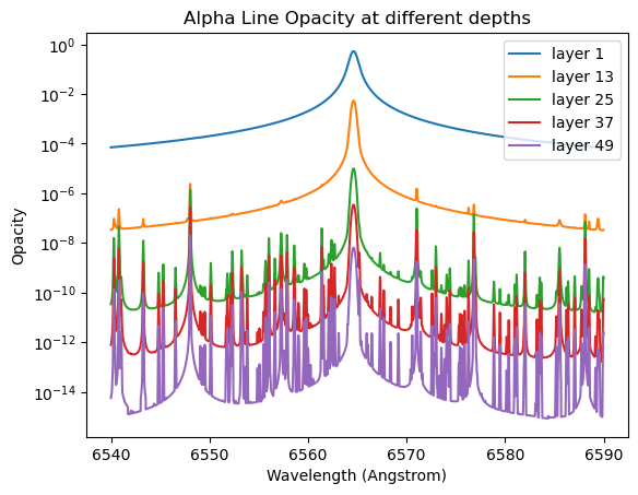
The stellar radiation field contains information on how light interacts with your star’s atmosphere in the simulation. The example below demonstrates sim.stellar_radiation_field.opacities.opacities_dict which contains a dictionary of each source of opacity and how much it contributes to the overall opacity at each wavelength at each depth.
This is a breakdown of how opacities_dict stores this information
opacities_dict['opacity_source'][depth_point_index, wavelength_index]
[ ]:
alpha_lines = sim.stellar_radiation_field.opacities.opacities_dict['alpha_line_at_nu']

for depth_point in range(1, len(alpha_lines), 12):

    plt.plot(sim.lambdas, alpha_lines[depth_point], label=f'layer {depth_point}')
plt.xlabel('Wavelength (Angstrom)')
plt.ylabel('Opacity')
plt.title('Alpha Line Opacity at different depths')
plt.legend()
plt.yscale('log')
array([[1.19396613e-04, 1.19494544e-04, 1.19592622e-04, ...,
        1.14524418e-04, 1.14429656e-04, 1.14335151e-04],
       [7.09791352e-05, 7.10375408e-05, 7.10960379e-05, ...,
        6.80940449e-05, 6.80365774e-05, 6.79793243e-05],
       [4.17916048e-05, 4.18262293e-05, 4.18609110e-05, ...,
        4.00929725e-05, 4.00584543e-05, 4.00241044e-05],
       ...,
       [6.53995312e-17, 6.55267275e-17, 6.56543559e-17, ...,
        5.56712932e-13, 5.44563628e-13, 4.43041798e-13],
       [2.54061313e-17, 2.54694767e-17, 2.55330590e-17, ...,
        3.73815457e-13, 3.65601935e-13, 2.97017936e-13],
       [1.43116146e-17, 1.43472978e-17, 1.43831146e-17, ...,
        2.47687524e-13, 2.42214851e-13, 1.96544874e-13]])
