You can interact with this notebook online: Launch notebook
How to Generate a Spectral element DEComposition (SDEC) Plot
The SDEC Plot illustrates the contributions of different chemical elements in the formation of a simulation model’s spectrum. It is a spectral diagnostic plot similar to those originally proposed by M. Kromer (see, for example, Kromer et al. 2013, figure 4).
First, create and run a simulation for which you want to generate this plot:
[2]:
from tardis import run_tardis
from tardis.io.atom_data import download_atom_data
# We download the atomic data needed to run the simulation
download_atom_data('kurucz_cd23_chianti_H_He')
sim = run_tardis("tardis_example.yml", virtual_packet_logging=True)
Atomic Data kurucz_cd23_chianti_H_He already exists in /home/runner/Downloads/tardis-data/kurucz_cd23_chianti_H_He.h5. Will not download - override with force_download=True.
[tardis.io.model.parse_atom_data][INFO ]
Reading Atomic Data from kurucz_cd23_chianti_H_He.h5 (parse_atom_data.py:40)
[tardis.io.atom_data.util][INFO ]
Atom Data kurucz_cd23_chianti_H_He.h5 not found in local path.
Exists in TARDIS Data repo /home/runner/Downloads/tardis-data/kurucz_cd23_chianti_H_He.h5 (util.py:34)
[tardis.io.atom_data.base][INFO ]
Reading Atom Data with: UUID = 6f7b09e887a311e7a06b246e96350010 MD5 = 864f1753714343c41f99cb065710cace (base.py:258)
[tardis.io.atom_data.base][INFO ]
Non provided Atomic Data: synpp_refs, photoionization_data, yg_data, two_photon_data, linelist_atoms, linelist_molecules (base.py:262)
[tardis.io.model.parse_density_configuration][WARNING]
Number of density points larger than number of shells. Assuming inner point irrelevant (parse_density_configuration.py:114)
[tardis.model.matter.decay][INFO ]
Decaying abundances for 1123200.0 seconds (decay.py:101)
[tardis.simulation.base][INFO ]
Starting iteration 1 of 20 (base.py:444)
[tardis.simulation.base][INFO ]
Luminosity emitted = 7.942e+42 erg / s
Luminosity absorbed = 2.659e+42 erg / s
Luminosity requested = 1.059e+43 erg / s
(base.py:657)
[tardis.simulation.base][INFO ]
Plasma stratification: (base.py:625)
| Shell No. | t_rad | next_t_rad | w | next_w |
|---|---|---|---|---|
| 0 | 9.93e+03 K | 1.01e+04 K | 0.4 | 0.507 |
| 5 | 9.85e+03 K | 1.02e+04 K | 0.211 | 0.197 |
| 10 | 9.78e+03 K | 1.01e+04 K | 0.143 | 0.117 |
| 15 | 9.71e+03 K | 9.87e+03 K | 0.105 | 0.0869 |
[tardis.simulation.base][INFO ]
Current t_inner = 9933.952 K
Expected t_inner for next iteration = 10703.212 K
(base.py:652)
[tardis.simulation.base][INFO ]
Starting iteration 2 of 20 (base.py:444)
[tardis.simulation.base][INFO ]
Luminosity emitted = 1.071e+43 erg / s
Luminosity absorbed = 3.576e+42 erg / s
Luminosity requested = 1.059e+43 erg / s
(base.py:657)
[tardis.simulation.base][INFO ]
Plasma stratification: (base.py:625)
| Shell No. | t_rad | next_t_rad | w | next_w |
|---|---|---|---|---|
| 0 | 1.01e+04 K | 1.08e+04 K | 0.507 | 0.525 |
| 5 | 1.02e+04 K | 1.1e+04 K | 0.197 | 0.203 |
| 10 | 1.01e+04 K | 1.08e+04 K | 0.117 | 0.125 |
| 15 | 9.87e+03 K | 1.05e+04 K | 0.0869 | 0.0933 |
[tardis.simulation.base][INFO ]
Current t_inner = 10703.212 K
Expected t_inner for next iteration = 10673.712 K
(base.py:652)
[tardis.simulation.base][INFO ]
Starting iteration 3 of 20 (base.py:444)
[tardis.simulation.base][INFO ]
Luminosity emitted = 1.074e+43 erg / s
Luminosity absorbed = 3.391e+42 erg / s
Luminosity requested = 1.059e+43 erg / s
(base.py:657)
[tardis.simulation.base][INFO ]
Iteration converged 1/4 consecutive times. (base.py:260)
[tardis.simulation.base][INFO ]
Plasma stratification: (base.py:625)
| Shell No. | t_rad | next_t_rad | w | next_w |
|---|---|---|---|---|
| 0 | 1.08e+04 K | 1.1e+04 K | 0.525 | 0.483 |
| 5 | 1.1e+04 K | 1.12e+04 K | 0.203 | 0.189 |
| 10 | 1.08e+04 K | 1.1e+04 K | 0.125 | 0.118 |
| 15 | 1.05e+04 K | 1.06e+04 K | 0.0933 | 0.0895 |
[tardis.simulation.base][INFO ]
Current t_inner = 10673.712 K
Expected t_inner for next iteration = 10635.953 K
(base.py:652)
[tardis.simulation.base][INFO ]
Starting iteration 4 of 20 (base.py:444)
[tardis.simulation.base][INFO ]
Luminosity emitted = 1.058e+43 erg / s
Luminosity absorbed = 3.352e+42 erg / s
Luminosity requested = 1.059e+43 erg / s
(base.py:657)
[tardis.simulation.base][INFO ]
Iteration converged 2/4 consecutive times. (base.py:260)
[tardis.simulation.base][INFO ]
Plasma stratification: (base.py:625)
| Shell No. | t_rad | next_t_rad | w | next_w |
|---|---|---|---|---|
| 0 | 1.1e+04 K | 1.1e+04 K | 0.483 | 0.469 |
| 5 | 1.12e+04 K | 1.12e+04 K | 0.189 | 0.182 |
| 10 | 1.1e+04 K | 1.1e+04 K | 0.118 | 0.113 |
| 15 | 1.06e+04 K | 1.07e+04 K | 0.0895 | 0.0861 |
[tardis.simulation.base][INFO ]
Current t_inner = 10635.953 K
Expected t_inner for next iteration = 10638.407 K
(base.py:652)
[tardis.simulation.base][INFO ]
Starting iteration 5 of 20 (base.py:444)
[tardis.simulation.base][INFO ]
Luminosity emitted = 1.055e+43 erg / s
Luminosity absorbed = 3.399e+42 erg / s
Luminosity requested = 1.059e+43 erg / s
(base.py:657)
[tardis.simulation.base][INFO ]
Iteration converged 3/4 consecutive times. (base.py:260)
[tardis.simulation.base][INFO ]
Plasma stratification: (base.py:625)
| Shell No. | t_rad | next_t_rad | w | next_w |
|---|---|---|---|---|
| 0 | 1.1e+04 K | 1.1e+04 K | 0.469 | 0.479 |
| 5 | 1.12e+04 K | 1.13e+04 K | 0.182 | 0.178 |
| 10 | 1.1e+04 K | 1.1e+04 K | 0.113 | 0.113 |
| 15 | 1.07e+04 K | 1.07e+04 K | 0.0861 | 0.0839 |
[tardis.simulation.base][INFO ]
Current t_inner = 10638.407 K
Expected t_inner for next iteration = 10650.202 K
(base.py:652)
[tardis.simulation.base][INFO ]
Starting iteration 6 of 20 (base.py:444)
[tardis.simulation.base][INFO ]
Luminosity emitted = 1.061e+43 erg / s
Luminosity absorbed = 3.398e+42 erg / s
Luminosity requested = 1.059e+43 erg / s
(base.py:657)
[tardis.simulation.base][INFO ]
Iteration converged 4/4 consecutive times. (base.py:260)
[tardis.simulation.base][INFO ]
Plasma stratification: (base.py:625)
| Shell No. | t_rad | next_t_rad | w | next_w |
|---|---|---|---|---|
| 0 | 1.1e+04 K | 1.1e+04 K | 0.479 | 0.47 |
| 5 | 1.13e+04 K | 1.12e+04 K | 0.178 | 0.185 |
| 10 | 1.1e+04 K | 1.11e+04 K | 0.113 | 0.112 |
| 15 | 1.07e+04 K | 1.07e+04 K | 0.0839 | 0.0856 |
[tardis.simulation.base][INFO ]
Current t_inner = 10650.202 K
Expected t_inner for next iteration = 10645.955 K
(base.py:652)
[tardis.simulation.base][INFO ]
Starting iteration 7 of 20 (base.py:444)
[tardis.simulation.base][INFO ]
Luminosity emitted = 1.061e+43 erg / s
Luminosity absorbed = 3.382e+42 erg / s
Luminosity requested = 1.059e+43 erg / s
(base.py:657)
[tardis.simulation.base][INFO ]
Iteration converged 5/4 consecutive times. (base.py:260)
[tardis.simulation.base][INFO ]
Plasma stratification: (base.py:625)
| Shell No. | t_rad | next_t_rad | w | next_w |
|---|---|---|---|---|
| 0 | 1.1e+04 K | 1.1e+04 K | 0.47 | 0.47 |
| 5 | 1.12e+04 K | 1.13e+04 K | 0.185 | 0.178 |
| 10 | 1.11e+04 K | 1.11e+04 K | 0.112 | 0.112 |
| 15 | 1.07e+04 K | 1.07e+04 K | 0.0856 | 0.086 |
[tardis.simulation.base][INFO ]
Current t_inner = 10645.955 K
Expected t_inner for next iteration = 10642.050 K
(base.py:652)
[tardis.simulation.base][INFO ]
Starting iteration 8 of 20 (base.py:444)
[tardis.simulation.base][INFO ]
Luminosity emitted = 1.062e+43 erg / s
Luminosity absorbed = 3.350e+42 erg / s
Luminosity requested = 1.059e+43 erg / s
(base.py:657)
[tardis.simulation.base][INFO ]
Iteration converged 6/4 consecutive times. (base.py:260)
[tardis.simulation.base][INFO ]
Plasma stratification: (base.py:625)
| Shell No. | t_rad | next_t_rad | w | next_w |
|---|---|---|---|---|
| 0 | 1.1e+04 K | 1.11e+04 K | 0.47 | 0.472 |
| 5 | 1.13e+04 K | 1.14e+04 K | 0.178 | 0.175 |
| 10 | 1.11e+04 K | 1.11e+04 K | 0.112 | 0.111 |
| 15 | 1.07e+04 K | 1.07e+04 K | 0.086 | 0.084 |
[tardis.simulation.base][INFO ]
Current t_inner = 10642.050 K
Expected t_inner for next iteration = 10636.106 K
(base.py:652)
[tardis.simulation.base][INFO ]
Starting iteration 9 of 20 (base.py:444)
[tardis.simulation.base][INFO ]
Luminosity emitted = 1.052e+43 erg / s
Luminosity absorbed = 3.411e+42 erg / s
Luminosity requested = 1.059e+43 erg / s
(base.py:657)
[tardis.simulation.base][INFO ]
Iteration converged 7/4 consecutive times. (base.py:260)
[tardis.simulation.base][INFO ]
Plasma stratification: (base.py:625)
| Shell No. | t_rad | next_t_rad | w | next_w |
|---|---|---|---|---|
| 0 | 1.11e+04 K | 1.11e+04 K | 0.472 | 0.469 |
| 5 | 1.14e+04 K | 1.15e+04 K | 0.175 | 0.17 |
| 10 | 1.11e+04 K | 1.11e+04 K | 0.111 | 0.109 |
| 15 | 1.07e+04 K | 1.08e+04 K | 0.084 | 0.0822 |
[tardis.simulation.base][INFO ]
Current t_inner = 10636.106 K
Expected t_inner for next iteration = 10654.313 K
(base.py:652)
[tardis.simulation.base][INFO ]
Starting iteration 10 of 20 (base.py:444)
[tardis.simulation.base][INFO ]
Luminosity emitted = 1.070e+43 erg / s
Luminosity absorbed = 3.335e+42 erg / s
Luminosity requested = 1.059e+43 erg / s
(base.py:657)
[tardis.simulation.base][INFO ]
Iteration converged 8/4 consecutive times. (base.py:260)
[tardis.simulation.base][INFO ]
Plasma stratification: (base.py:625)
| Shell No. | t_rad | next_t_rad | w | next_w |
|---|---|---|---|---|
| 0 | 1.11e+04 K | 1.1e+04 K | 0.469 | 0.475 |
| 5 | 1.15e+04 K | 1.14e+04 K | 0.17 | 0.177 |
| 10 | 1.11e+04 K | 1.11e+04 K | 0.109 | 0.112 |
| 15 | 1.08e+04 K | 1.06e+04 K | 0.0822 | 0.0878 |
[tardis.simulation.base][INFO ]
Current t_inner = 10654.313 K
Expected t_inner for next iteration = 10628.190 K
(base.py:652)
[tardis.simulation.base][INFO ]
Starting iteration 11 of 20 (base.py:444)
[tardis.simulation.base][INFO ]
Luminosity emitted = 1.053e+43 erg / s
Luminosity absorbed = 3.363e+42 erg / s
Luminosity requested = 1.059e+43 erg / s
(base.py:657)
[tardis.simulation.base][INFO ]
Iteration converged 9/4 consecutive times. (base.py:260)
[tardis.simulation.base][INFO ]
Plasma stratification: (base.py:625)
| Shell No. | t_rad | next_t_rad | w | next_w |
|---|---|---|---|---|
| 0 | 1.1e+04 K | 1.1e+04 K | 0.475 | 0.472 |
| 5 | 1.14e+04 K | 1.12e+04 K | 0.177 | 0.184 |
| 10 | 1.11e+04 K | 1.1e+04 K | 0.112 | 0.114 |
| 15 | 1.06e+04 K | 1.06e+04 K | 0.0878 | 0.0859 |
[tardis.simulation.base][INFO ]
Current t_inner = 10628.190 K
Expected t_inner for next iteration = 10644.054 K
(base.py:652)
[tardis.simulation.base][INFO ]
Starting iteration 12 of 20 (base.py:444)
[tardis.simulation.base][INFO ]
Luminosity emitted = 1.056e+43 erg / s
Luminosity absorbed = 3.420e+42 erg / s
Luminosity requested = 1.059e+43 erg / s
(base.py:657)
[tardis.simulation.base][INFO ]
Iteration converged 10/4 consecutive times. (base.py:260)
[tardis.simulation.base][INFO ]
Plasma stratification: (base.py:625)
| Shell No. | t_rad | next_t_rad | w | next_w |
|---|---|---|---|---|
| 0 | 1.1e+04 K | 1.11e+04 K | 0.472 | 0.467 |
| 5 | 1.12e+04 K | 1.13e+04 K | 0.184 | 0.176 |
| 10 | 1.1e+04 K | 1.11e+04 K | 0.114 | 0.11 |
| 15 | 1.06e+04 K | 1.08e+04 K | 0.0859 | 0.0821 |
[tardis.simulation.base][INFO ]
Current t_inner = 10644.054 K
Expected t_inner for next iteration = 10653.543 K
(base.py:652)
[tardis.simulation.base][INFO ]
Starting iteration 13 of 20 (base.py:444)
[tardis.simulation.base][INFO ]
Luminosity emitted = 1.062e+43 erg / s
Luminosity absorbed = 3.406e+42 erg / s
Luminosity requested = 1.059e+43 erg / s
(base.py:657)
[tardis.simulation.base][INFO ]
Iteration converged 11/4 consecutive times. (base.py:260)
[tardis.simulation.base][INFO ]
Plasma stratification: (base.py:625)
| Shell No. | t_rad | next_t_rad | w | next_w |
|---|---|---|---|---|
| 0 | 1.11e+04 K | 1.11e+04 K | 0.467 | 0.466 |
| 5 | 1.13e+04 K | 1.13e+04 K | 0.176 | 0.18 |
| 10 | 1.11e+04 K | 1.11e+04 K | 0.11 | 0.111 |
| 15 | 1.08e+04 K | 1.08e+04 K | 0.0821 | 0.0841 |
[tardis.simulation.base][INFO ]
Current t_inner = 10653.543 K
Expected t_inner for next iteration = 10647.277 K
(base.py:652)
[tardis.simulation.base][INFO ]
Starting iteration 14 of 20 (base.py:444)
[tardis.simulation.base][INFO ]
Luminosity emitted = 1.063e+43 erg / s
Luminosity absorbed = 3.369e+42 erg / s
Luminosity requested = 1.059e+43 erg / s
(base.py:657)
[tardis.simulation.base][INFO ]
Iteration converged 12/4 consecutive times. (base.py:260)
[tardis.simulation.base][INFO ]
Plasma stratification: (base.py:625)
| Shell No. | t_rad | next_t_rad | w | next_w |
|---|---|---|---|---|
| 0 | 1.11e+04 K | 1.11e+04 K | 0.466 | 0.469 |
| 5 | 1.13e+04 K | 1.13e+04 K | 0.18 | 0.182 |
| 10 | 1.11e+04 K | 1.1e+04 K | 0.111 | 0.113 |
| 15 | 1.08e+04 K | 1.07e+04 K | 0.0841 | 0.0854 |
[tardis.simulation.base][INFO ]
Current t_inner = 10647.277 K
Expected t_inner for next iteration = 10638.875 K
(base.py:652)
[tardis.simulation.base][INFO ]
Starting iteration 15 of 20 (base.py:444)
[tardis.simulation.base][INFO ]
Luminosity emitted = 1.053e+43 erg / s
Luminosity absorbed = 3.417e+42 erg / s
Luminosity requested = 1.059e+43 erg / s
(base.py:657)
[tardis.simulation.base][INFO ]
Iteration converged 13/4 consecutive times. (base.py:260)
[tardis.simulation.base][INFO ]
Plasma stratification: (base.py:625)
| Shell No. | t_rad | next_t_rad | w | next_w |
|---|---|---|---|---|
| 0 | 1.11e+04 K | 1.1e+04 K | 0.469 | 0.484 |
| 5 | 1.13e+04 K | 1.13e+04 K | 0.182 | 0.181 |
| 10 | 1.1e+04 K | 1.1e+04 K | 0.113 | 0.113 |
| 15 | 1.07e+04 K | 1.07e+04 K | 0.0854 | 0.0858 |
[tardis.simulation.base][INFO ]
Current t_inner = 10638.875 K
Expected t_inner for next iteration = 10655.125 K
(base.py:652)
[tardis.simulation.base][INFO ]
Starting iteration 16 of 20 (base.py:444)
[tardis.simulation.base][INFO ]
Luminosity emitted = 1.059e+43 erg / s
Luminosity absorbed = 3.445e+42 erg / s
Luminosity requested = 1.059e+43 erg / s
(base.py:657)
[tardis.simulation.base][INFO ]
Iteration converged 14/4 consecutive times. (base.py:260)
[tardis.simulation.base][INFO ]
Plasma stratification: (base.py:625)
| Shell No. | t_rad | next_t_rad | w | next_w |
|---|---|---|---|---|
| 0 | 1.1e+04 K | 1.1e+04 K | 0.484 | 0.472 |
| 5 | 1.13e+04 K | 1.13e+04 K | 0.181 | 0.177 |
| 10 | 1.1e+04 K | 1.1e+04 K | 0.113 | 0.113 |
| 15 | 1.07e+04 K | 1.06e+04 K | 0.0858 | 0.0858 |
[tardis.simulation.base][INFO ]
Current t_inner = 10655.125 K
Expected t_inner for next iteration = 10655.561 K
(base.py:652)
[tardis.simulation.base][INFO ]
Starting iteration 17 of 20 (base.py:444)
[tardis.simulation.base][INFO ]
Luminosity emitted = 1.067e+43 erg / s
Luminosity absorbed = 3.372e+42 erg / s
Luminosity requested = 1.059e+43 erg / s
(base.py:657)
[tardis.simulation.base][INFO ]
Iteration converged 15/4 consecutive times. (base.py:260)
[tardis.simulation.base][INFO ]
Plasma stratification: (base.py:625)
| Shell No. | t_rad | next_t_rad | w | next_w |
|---|---|---|---|---|
| 0 | 1.1e+04 K | 1.11e+04 K | 0.472 | 0.468 |
| 5 | 1.13e+04 K | 1.14e+04 K | 0.177 | 0.175 |
| 10 | 1.1e+04 K | 1.11e+04 K | 0.113 | 0.11 |
| 15 | 1.06e+04 K | 1.08e+04 K | 0.0858 | 0.0816 |
[tardis.simulation.base][INFO ]
Current t_inner = 10655.561 K
Expected t_inner for next iteration = 10636.536 K
(base.py:652)
[tardis.simulation.base][INFO ]
Starting iteration 18 of 20 (base.py:444)
[tardis.simulation.base][INFO ]
Luminosity emitted = 1.057e+43 erg / s
Luminosity absorbed = 3.365e+42 erg / s
Luminosity requested = 1.059e+43 erg / s
(base.py:657)
[tardis.simulation.base][INFO ]
Iteration converged 16/4 consecutive times. (base.py:260)
[tardis.simulation.base][INFO ]
Plasma stratification: (base.py:625)
| Shell No. | t_rad | next_t_rad | w | next_w |
|---|---|---|---|---|
| 0 | 1.11e+04 K | 1.11e+04 K | 0.468 | 0.464 |
| 5 | 1.14e+04 K | 1.13e+04 K | 0.175 | 0.177 |
| 10 | 1.11e+04 K | 1.1e+04 K | 0.11 | 0.113 |
| 15 | 1.08e+04 K | 1.07e+04 K | 0.0816 | 0.0848 |
[tardis.simulation.base][INFO ]
Current t_inner = 10636.536 K
Expected t_inner for next iteration = 10641.692 K
(base.py:652)
[tardis.simulation.base][INFO ]
Starting iteration 19 of 20 (base.py:444)
[tardis.simulation.base][INFO ]
Luminosity emitted = 1.056e+43 erg / s
Luminosity absorbed = 3.405e+42 erg / s
Luminosity requested = 1.059e+43 erg / s
(base.py:657)
[tardis.simulation.base][INFO ]
Iteration converged 17/4 consecutive times. (base.py:260)
[tardis.simulation.base][INFO ]
Plasma stratification: (base.py:625)
| Shell No. | t_rad | next_t_rad | w | next_w |
|---|---|---|---|---|
| 0 | 1.11e+04 K | 1.11e+04 K | 0.464 | 0.466 |
| 5 | 1.13e+04 K | 1.13e+04 K | 0.177 | 0.177 |
| 10 | 1.1e+04 K | 1.11e+04 K | 0.113 | 0.111 |
| 15 | 1.07e+04 K | 1.07e+04 K | 0.0848 | 0.0853 |
[tardis.simulation.base][INFO ]
Current t_inner = 10641.692 K
Expected t_inner for next iteration = 10650.463 K
(base.py:652)
[tardis.simulation.base][INFO ]
Simulation finished in 19 iterations
Simulation took 51.48 s
(base.py:542)
[tardis.simulation.base][INFO ]
Starting iteration 20 of 20 (base.py:444)
[tardis.simulation.base][INFO ]
Luminosity emitted = 1.061e+43 erg / s
Luminosity absorbed = 3.401e+42 erg / s
Luminosity requested = 1.059e+43 erg / s
(base.py:657)
Note
The virtual packet logging capability must be active in order to produce the SDEC Plot for virtual packets population. Thus, make sure to set virtual_packet_logging: True in your configuration file if you want to generate the SDEC Plot with virtual packets. It should be added under the virtual property of the spectrum property, as described in the configuration schema.
Now, import the plotting interface for the SDEC plot, i.e. the SDECPlotter class.
[3]:
from tardis.visualization import SDECPlotter
And create a plotter object to process the data of simulation object sim for generating the SDEC plots.
[4]:
plotter = SDECPlotter.from_simulation(sim)
Static Plot (in matplotlib)
You can now call the generate_plot_mpl() method on your plotter object to get a highly informative, yet beautiful, SDEC plot produced in matplotlib.
Virtual packets mode
By default, an SDEC plot is produced for the virtual packet population of the simulation.
[5]:
plotter.generate_plot_mpl()
[5]:
<Axes: xlabel='Wavelength $[\\mathrm{\\AA}]$', ylabel='$L_{\\lambda}$ [erg $\\mathrm{s^{-1}}$ $\\mathrm{\\AA^{-1}}$]'>

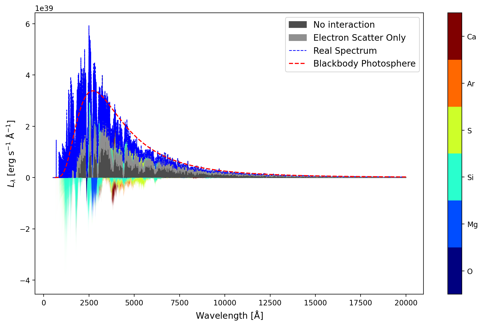
Real packets mode
You can produce the SDEC plot for the real packet population of the simulation by setting packets_mode="real" which is "virtual" by default. Since packets_mode is the 1st argument, you can simply pass "real" string only.
[6]:
plotter.generate_plot_mpl("real")
[6]:
<Axes: xlabel='Wavelength $[\\mathrm{\\AA}]$', ylabel='$L_{\\lambda}$ [erg $\\mathrm{s^{-1}}$ $\\mathrm{\\AA^{-1}}$]'>
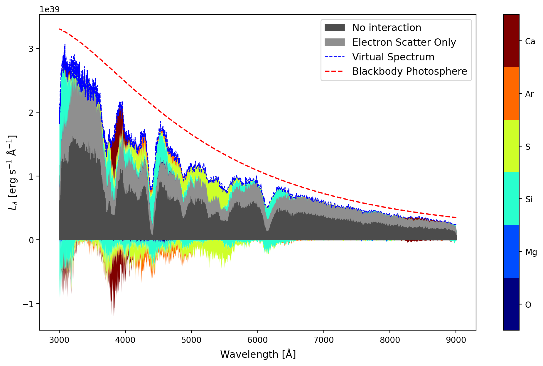
Plotting a specific wavelength range
You can also restrict the wavelength range of escaped packets that you want to plot by specifying packet_wvl_range. It should be a quantity in Angstroms, containing two values - lower lambda and upper lambda i.e. [lower_lambda, upper_lambda] * u.AA.
[7]:
from astropy import units as u
[8]:
plotter.generate_plot_mpl(packet_wvl_range=[3000, 9000] * u.AA)
[8]:
<Axes: xlabel='Wavelength $[\\mathrm{\\AA}]$', ylabel='$L_{\\lambda}$ [erg $\\mathrm{s^{-1}}$ $\\mathrm{\\AA^{-1}}$]'>
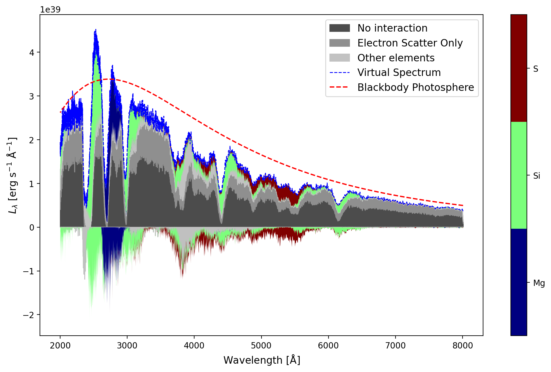
Plotting only the top contributing elements
The nelements option allows you to plot the top contributing elements to the spectrum. The top elements are shown in unique colors and the rest of the elements are shown in silver. Please note this works only for elements and not for ions.
[9]:
plotter.generate_plot_mpl(packet_wvl_range=[2000, 8000] * u.AA, nelements = 3)
[9]:
<Axes: xlabel='Wavelength $[\\mathrm{\\AA}]$', ylabel='$L_{\\lambda}$ [erg $\\mathrm{s^{-1}}$ $\\mathrm{\\AA^{-1}}$]'>
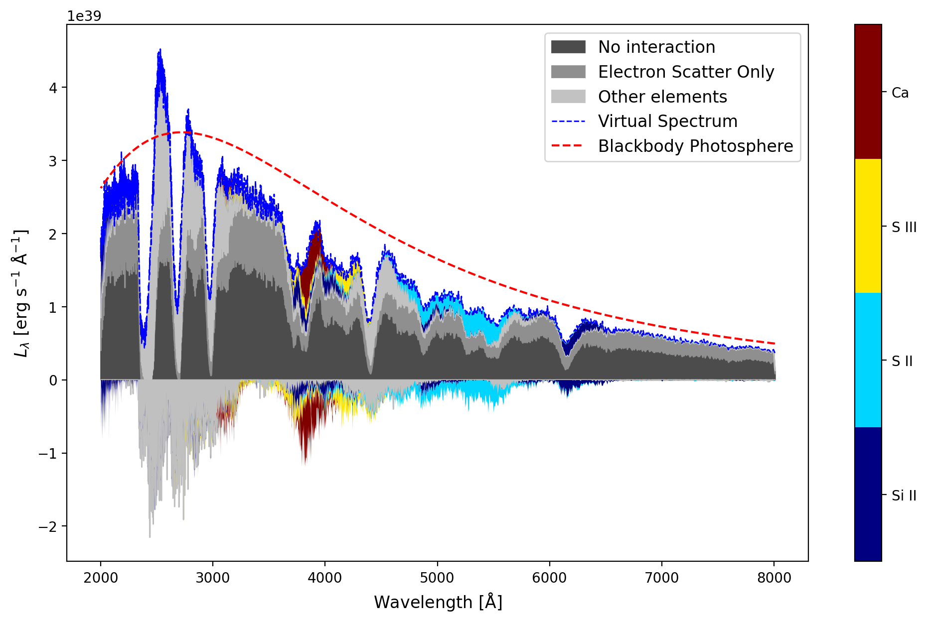
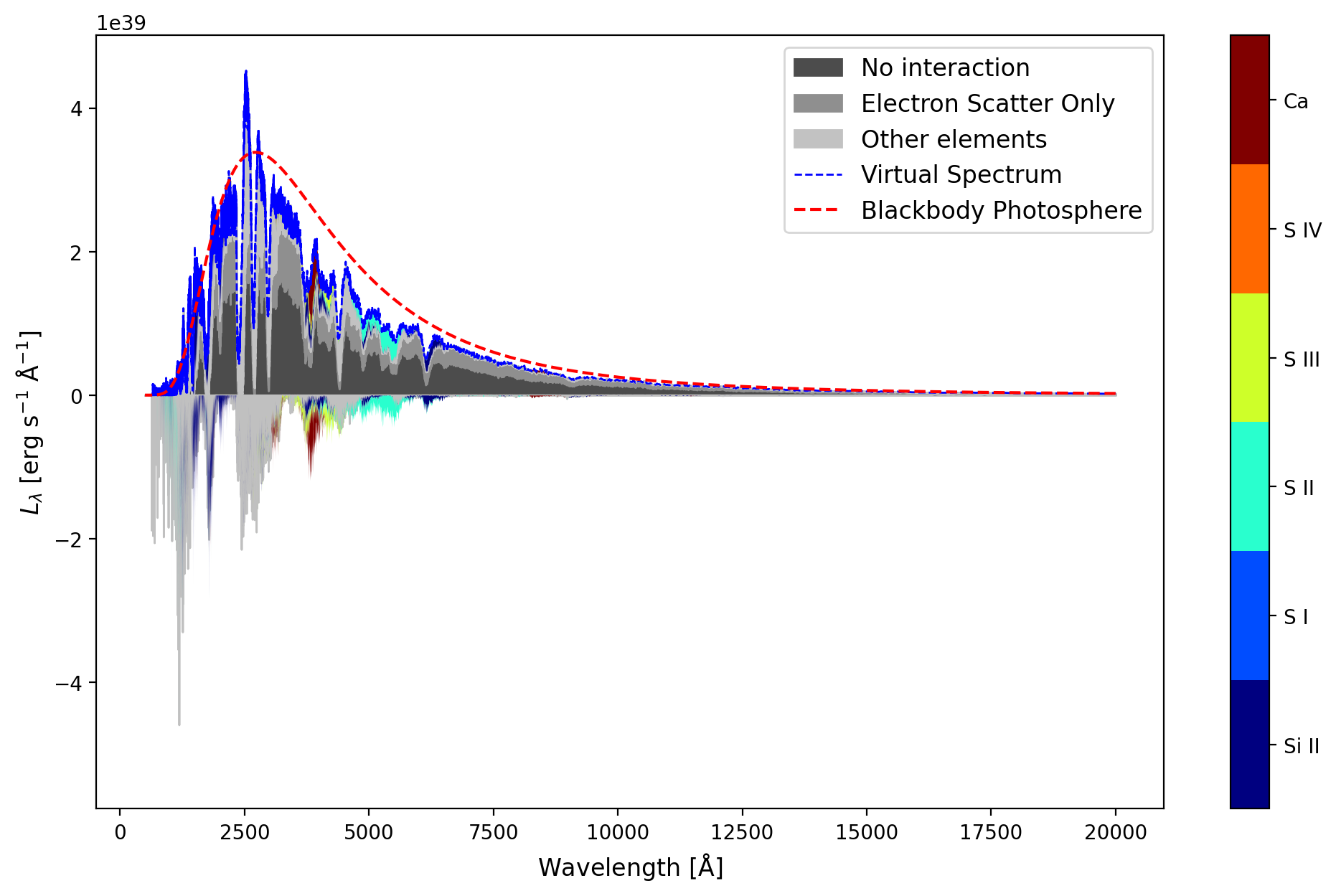
Choosing what elements/ions to plot
You can also pass a list of elements/ions of your choice in the species_list option and plot them. Valid options include elements (e.g. Si), ions (which must be specified in Roman numeral format, e.g. Si II), a range of ions (e.g. Si I-III), or any combination of these.
[10]:
plotter.generate_plot_mpl(packet_wvl_range=[2000, 8000] * u.AA, species_list = ['Si II', 'S I-V', 'Ca'])
[10]:
<Axes: xlabel='Wavelength $[\\mathrm{\\AA}]$', ylabel='$L_{\\lambda}$ [erg $\\mathrm{s^{-1}}$ $\\mathrm{\\AA^{-1}}$]'>
When using both the nelements and the species_list options, species_list takes precedence.
[11]:
plotter.generate_plot_mpl(nelements = 3, species_list = ['Si II', 'S I-V', 'Ca'])
[tardis.visualization.tools.sdec_plot][INFO ]
Both nelements and species_list were requested. Species_list takes priority; nelements is ignored (sdec_plot.py:1208)
[11]:
<Axes: xlabel='Wavelength $[\\mathrm{\\AA}]$', ylabel='$L_{\\lambda}$ [erg $\\mathrm{s^{-1}}$ $\\mathrm{\\AA^{-1}}$]'>
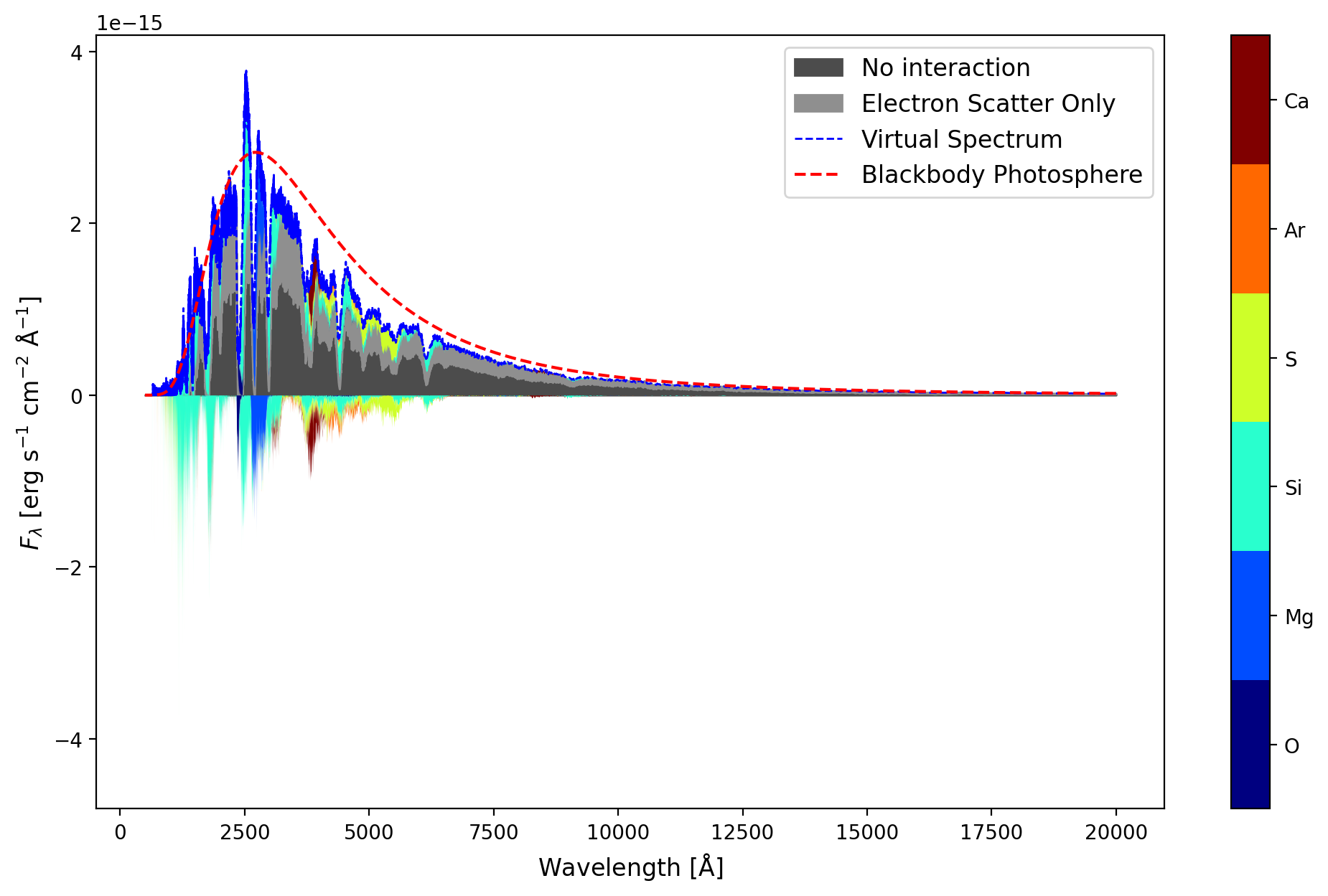
Plotting flux instead of luminosity
You can plot in units of flux on the Y-axis of the SDEC plot, by specifying the distance parameter. It should be a quantity with a unit of length like m, Mpc, etc. and must be a positive value. By default, distance=None plots luminosity on the Y-axis.
[12]:
plotter.generate_plot_mpl(distance=100 * u.Mpc)
[12]:
<Axes: xlabel='Wavelength $[\\mathrm{\\AA}]$', ylabel='$F_{\\lambda}$ [erg $\\mathrm{s^{-1}}$ $\\mathrm{cm^{-2}}$ $\\mathrm{\\AA^{-1}}$]'>
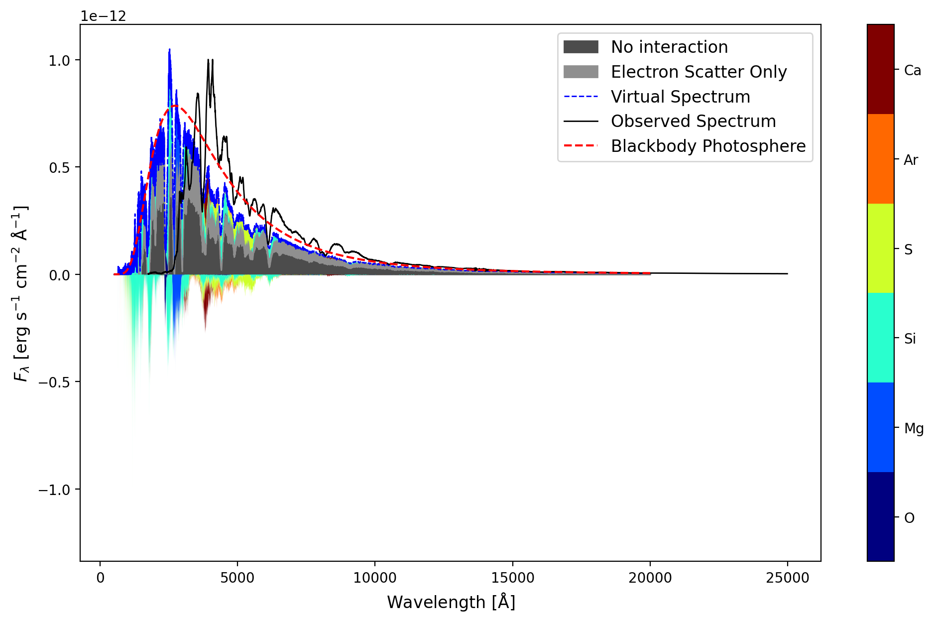
Plotting an observed spectrum
To add an observed spectrum to the SDEC plot, you would need to pass the wavelength and the flux to the observed_spectrum parameter. The argument passed should be a tuple/list where the first value is the wavelength and the second value is the flux of the observed spectrum. Please note that these values should be instances of astropy.Quantity.
[13]:
import numpy as np
data = np.loadtxt('demo_observed_spectrum.dat')
observed_spectrum_wavelength, observed_spectrum_flux = data.T
observed_spectrum_wavelength = observed_spectrum_wavelength * u.AA
observed_spectrum_flux = observed_spectrum_flux * u.erg / (u.s * u.cm**2 * u.AA)
[14]:
plotter.generate_plot_mpl(observed_spectrum = (observed_spectrum_wavelength, observed_spectrum_flux), distance = 6 * u.Mpc)
[14]:
<Axes: xlabel='Wavelength $[\\mathrm{\\AA}]$', ylabel='$F_{\\lambda}$ [erg $\\mathrm{s^{-1}}$ $\\mathrm{cm^{-2}}$ $\\mathrm{\\AA^{-1}}$]'>
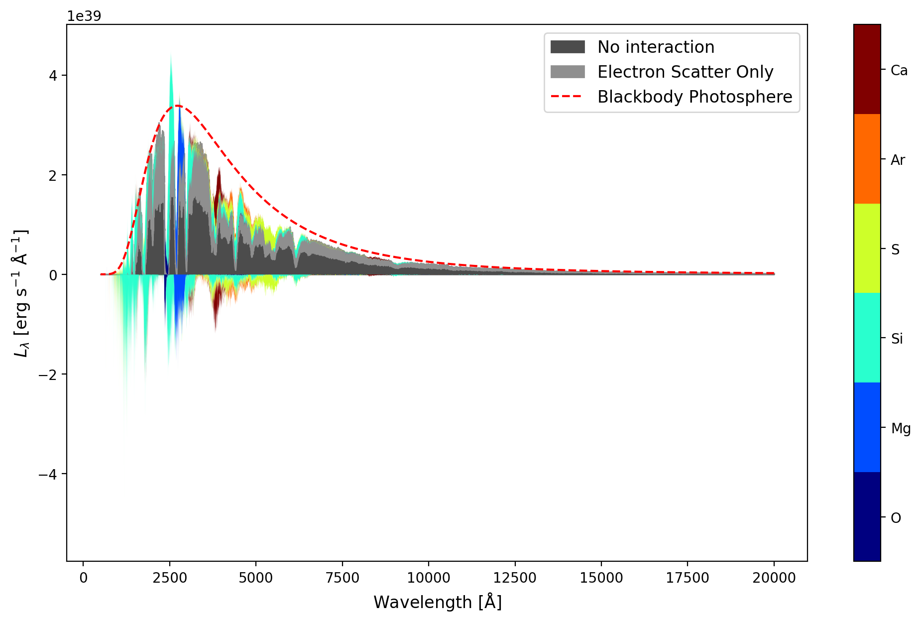
Hiding modeled spectrum
By default, the modeled spectrum is shown in SDEC plot. You can hide it by setting show_modeled_spectrum=False.
[15]:
plotter.generate_plot_mpl(show_modeled_spectrum=False)
[15]:
<Axes: xlabel='Wavelength $[\\mathrm{\\AA}]$', ylabel='$L_{\\lambda}$ [erg $\\mathrm{s^{-1}}$ $\\mathrm{\\AA^{-1}}$]'>
Additional plotting options
[16]:
# To list all available options (or parameters) with their description
help(plotter.generate_plot_mpl)
Help on method generate_plot_mpl in module tardis.visualization.tools.sdec_plot:
generate_plot_mpl(packets_mode='virtual', packet_wvl_range=None, distance=None, observed_spectrum=None, show_modeled_spectrum=True, ax=None, figsize=(12, 7), cmapname='jet', nelements=None, species_list=None, blackbody_photosphere=True) method of tardis.visualization.tools.sdec_plot.SDECPlotter instance
Generate Spectral element DEComposition (SDEC) Plot using matplotlib.
Parameters
----------
packets_mode : {'virtual', 'real'}, optional
Mode of packets to be considered, either real or virtual. Default
value is 'virtual'
packet_wvl_range : astropy.Quantity or None, optional
Wavelength range to restrict the analysis of escaped packets. It
should be a quantity having units of Angstrom, containing two
values - lower lambda and upper lambda i.e.
[lower_lambda, upper_lambda] * u.AA. Default value is None
distance : astropy.Quantity or None, optional
Distance used to calculate flux instead of luminosity in the plot.
It should have a length unit like m, Mpc, etc. Default value is None
observed_spectrum : tuple or list of astropy.Quantity, optional
Option to plot an observed spectrum in the SDEC plot. If given, the first element
should be the wavelength and the second element should be flux,
i.e. (wavelength, flux). The assumed units for wavelength and flux are
angstroms and erg/(angstroms * s * cm^2), respectively. Default value is None.
show_modeled_spectrum : bool, optional
Whether to show modeled spectrum in SDEC Plot. Default value is
True
ax : matplotlib.axes._subplots.AxesSubplot or None, optional
Axis on which to create plot. Default value is None which will
create plot on a new figure's axis.
figsize : tuple, optional
Size of the matplotlib figure to display. Default value is (12, 7)
cmapname : str, optional
Name of matplotlib colormap to be used for showing elements.
Default value is "jet"
nelements: int
Number of elements to include in plot. Determined by the
largest contribution to total luminosity absorbed and emitted.
Other elements are shown in silver. Default value is
None, which displays all elements
species_list: list of strings or None
list of strings containing the names of species that should be included in the SDEC plots.
Must be given in Roman numeral format. Can include specific ions, a range of ions,
individual elements, or any combination of these:
e.g. ['Si II', 'Ca II', 'C', 'Fe I-V']
blackbody_photosphere: bool
Whether to include the blackbody photosphere in the plot. Default value is True
Returns
-------
matplotlib.axes._subplots.AxesSubplot
Axis on which SDEC Plot is created
The generate_plot_mpl method also has options specific to the matplotlib API, thereby providing you with more control over how your SDEC plot looks. Possible cases where you may use them are:
ax: To plot SDEC on the Axis of a plot you’re already working with, e.g. for subplots.figsize: To resize the SDEC plot as per your requirements.cmapname: To use a colormap of your preference, instead of “jet”.
Interactive Plot (in plotly)
If you’re using the SDEC plot for exploration purposes, you should plot its interactive version by using generate_plot_ply(). This not only allows you to zoom & pan but also to inspect data values by hovering, to resize scale, etc. conveniently (as shown below).
This method takes the exact same arguments as ``generate_plot_mpl`` except a few that are specific to the plotting library. We can produce all the plots above in plotly, by passing the same arguments.
Virtual packets mode
[17]:
plotter.generate_plot_ply()
Real packets mode
[18]:
plotter.generate_plot_ply(packets_mode="real")
In a similar manner, you can also use the packet_wvl_range, nelements, species_list, show_modeled_spectrum, observed_spectrum and distance arguments in plotly plots (try it out in interactive mode!).
Additional plotting options
The generate_plot_ply method also has options specific to the plotly API, thereby providing you with more control over how your SDEC plot looks. Possible cases where you may use them are: - fig: To plot the SDEC plot on a figure you are already using e.g. for subplots. - graph_height: To specify the height of the graph as needed. - cmapname: To use a colormap of your preference instead of “jet”.
[19]:
# To list all available options (or parameters) with their description
help(plotter.generate_plot_ply)
Help on method generate_plot_ply in module tardis.visualization.tools.sdec_plot:
generate_plot_ply(packets_mode='virtual', packet_wvl_range=None, distance=None, observed_spectrum=None, show_modeled_spectrum=True, fig=None, graph_height=600, cmapname='jet', nelements=None, species_list=None, blackbody_photosphere=True) method of tardis.visualization.tools.sdec_plot.SDECPlotter instance
Generate interactive Spectral element DEComposition (SDEC) Plot using plotly.
Parameters
----------
packets_mode : {'virtual', 'real'}, optional
Mode of packets to be considered, either real or virtual. Default
value is 'virtual'
packet_wvl_range : astropy.Quantity or None, optional
Wavelength range to restrict the analysis of escaped packets. It
should be a quantity having units of Angstrom, containing two
values - lower lambda and upper lambda i.e.
[lower_lambda, upper_lambda] * u.AA. Default value is None
distance : astropy.Quantity or None, optional
Distance used to calculate flux instead of luminosity in the plot.
It should have a length unit like m, Mpc, etc. Default value is None
observed_spectrum : tuple or list of astropy.Quantity, optional
Option to plot an observed spectrum in the SDEC plot. If given, the first element
should be the wavelength and the second element should be flux,
i.e. (wavelength, flux). The assumed units for wavelength and flux are
angstroms and erg/(angstroms * s * cm^2), respectively. Default value is None.
show_modeled_spectrum : bool, optional
Whether to show modeled spectrum in SDEC Plot. Default value is
True
fig : plotly.graph_objs._figure.Figure or None, optional
Figure object on which to create plot. Default value is None which
will create plot on a new Figure object.
graph_height : int, optional
Height (in px) of the plotly graph to display. Default value is 600
cmapname : str, optional
Name of the colormap to be used for showing elements.
Default value is "jet"
nelements: int
Number of elements to include in plot. Determined by the
largest contribution to total luminosity absorbed and emitted.
Other elements are shown in silver. Default value is
None, which displays all elements
species_list: list of strings or None
list of strings containing the names of species that should be included in the SDEC plots.
Must be given in Roman numeral format. Can include specific ions, a range of ions,
individual elements, or any combination of these:
e.g. ['Si II', 'Ca II', 'C', 'Fe I-V']
blackbody_photosphere: bool
Whether to include the blackbody photosphere in the plot. Default value is True
Returns
-------
plotly.graph_objs._figure.Figure
Figure object on which SDEC Plot is created
Using simulation saved as HDF
Other than producing the SDEC Plot for simulation objects in runtime, you can also produce it for saved TARDIS simulations.
[20]:
# hdf_plotter = SDECPlotter.from_hdf("demo.h5") ## Files is too large - just as an example
This hdf_plotter object is similar to the plotter object we used above, so you can use each plotting method demonstrated above with this too.
[21]:
# Static plot with virtual packets mode
# hdf_plotter.generate_plot_mpl()
[22]:
# Static plot with real packets mode
# hdf_plotter.generate_plot_mpl("real")
[23]:
# Interactive plot with virtual packets mode
# hdf_plotter.generate_plot_ply()