You can interact with this notebook online: Launch notebook

Custom Abundance Widget

The Custom Abundance Widget is a Graphical User Interface (GUI) that allows you to develop custom model compositions graphically and output the model to a new file — all within a Jupyter Notebook.

The GUI consists of three parts:

1. Visualization plot — An interactive step graph that shows abundances and densities as a function of velocity.

2. Data editor — An interface to edit abundances, densities, and velocity shells.

3. File output — An output module to save the model compositions as a CSVY file.

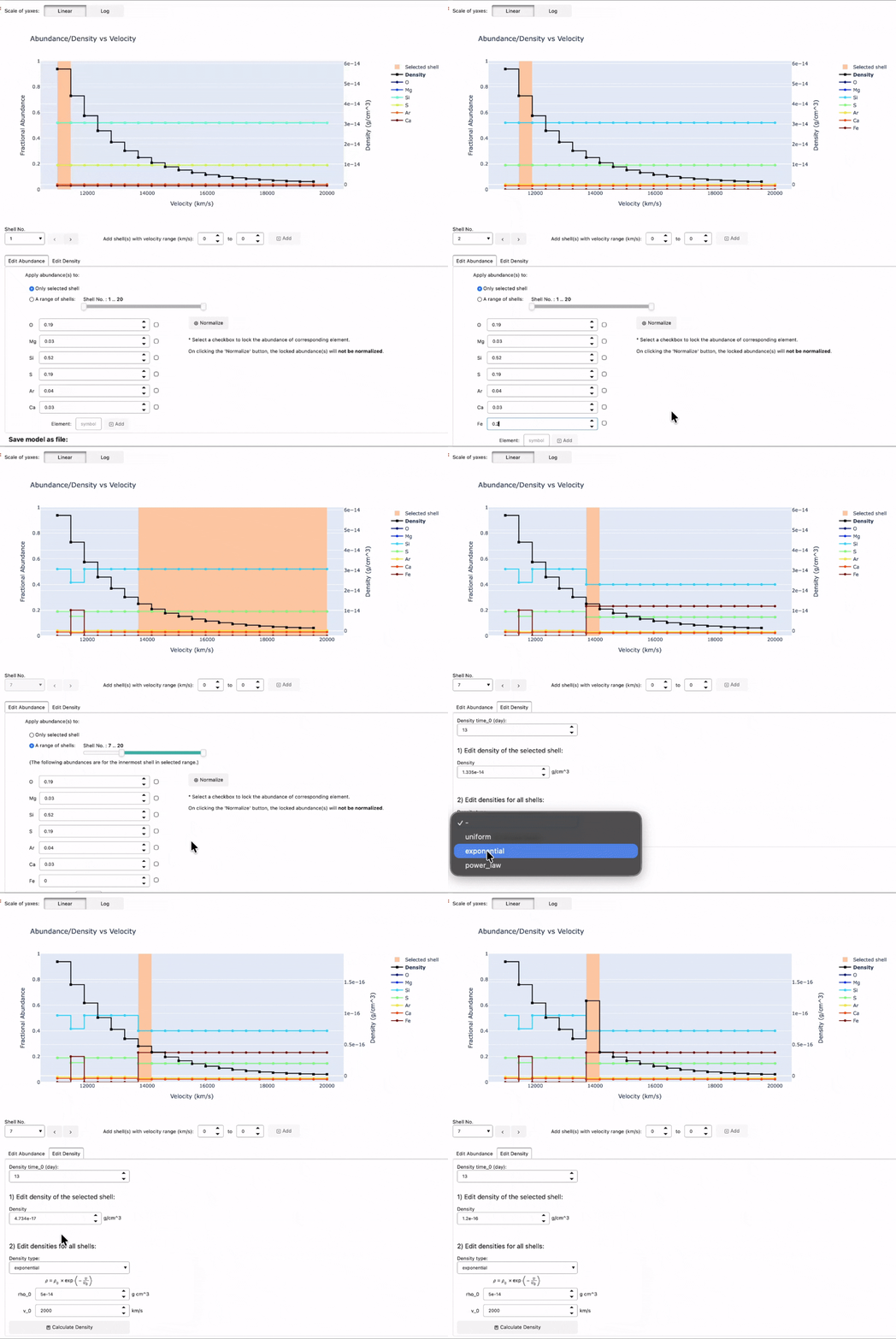
Interacting with the GUI

Edit Abundances

There are two radio buttons that let you edit either a single shell or multiple shells. The new input is applied to the selected shell(s) immediately and the plot updates at the same time. To edit multiple shells at once, choose the second radio button and set the range of shell numbers using the int slider. The selected shell(s) are highlighted in the plot.

Normalize Abundances

Click the Normalize button to normalize the abundances of the selected shell(s) to 1. To keep the abundance of a particular element unchanged during normalization, select the checkbox next to that element to lock it. The normalization is applied to the other elements so that the total still sums to 1.

Edit Densities

In the Edit Density tab, you can edit either a single shell or the whole density profile. Choose a density type and supply the required parameters to calculate a new profile.

Add a New Element

The symbol input box at the bottom of the editor lets you add a new element or isotope to the model. It automatically checks whether the symbol is valid and whether the element is already present in the model.

Add a New Shell

You can add a new shell to the model by specifying its velocity range. Abundances for the new shell are initialized to 0. Existing shells are resized automatically if the new shell overlaps with any of them.

Generating the Widget

Import CustomAbundanceWidget from the visualization subpackage to create the widget.

from tardis.visualization import CustomAbundanceWidget

Initializing tabulator and plotly panel extensions for widgets to work

There are four ways to initialize the widget. You can generate it from a .yml or .csvy configuration file before running any simulation, or from a Simulation object or saved HDF file after a simulation.

Warning

Custom abundance widget currently exhibits unintended behavior when run in a notebook where a simulation has already been run. It is recommended to run the widget in a fresh notebook without running any simulation first.

Using a YAML file

widget = CustomAbundanceWidget.from_yml("tardis_example.yml")

Number of density points larger than number of shells. Assuming inner point irrelevant
model_isotope_time_0 is not set in the configuration. Isotopic mass fractions will not be decayed and is assumed to be correct for the time_explosion. THIS IS NOT RECOMMENDED!

Using a CSVY File

# widget = CustomAbundanceWidget.from_csvy("demo.csvy")

Using a Simulation Object

# sim = run_tardis("tardis_example.yml")
# widget = CustomAbundanceWidget.from_simulation(sim)

Using an HDF File

# widget = CustomAbundanceWidget.from_hdf("demo.h5")

Display the Widget

Regardless of which initialization method you use, call .display() to render the GUI.

Note for Documentation Viewers

The interactive widget below will not function in the published documentation. To use this widget, please run this notebook locally in a Jupyter environment with TARDIS installed.

widget.display()